Comenius University,
Faculty of Mathematics, Physics and
Informatics,
Deartment of Computer Graphics
Procedural Textures Created
on Cellular Automata
Peter Borovsky
Bratislava, 2003
Slovakia
Keywords
procedural texture, texture
synthesis, cellular automaton, noise
Purpose
This document is written as rigorous
thesis in Computer Graphics applied at the Department of Computer
Graphics, FMFI UK. We want to show reader our view on texture synthesis. We are
generating 2D images with famous procedural texture algorithms as well as some
we invented ad hoc. In this document cellular Automata (CA) are chosen as a
tool for texture synthesis. Much of our work is available in digital form.
There are our programs, their sources and a little more accompanied to this
hardcopy.
Text and all figures in the document
are property of Peter Borovský.
Style
We did not want to overload reader
with definitions and theorem proofs, therefore we choose less formal style of written text.
Important term introduced first time is written in italics. We expect
reader is acknowledged with some part of the computer graphics.
Document is divided into 6 sections.
This is the introducting one. First section contains our categorization of texture
synthesis techiques. Second section gives an overview of texture synthesis
applications. Then comes short introduction to cellular automata. Our study of
CA follows in section 4 and 5. Appendices are marked as section 6.
Introduction
Texture synthesis, as well as overall
computer graphics, joins many aspects of art, natural sciences and engineering.
There is a theory background and, on the other side, there are practical
applications helping users to enjoy the world of artificial images.
We assume reader is acknowledged with
basics of texture synthesis. Anyway, we will mention some facts as for
beginners.
In our work, we are not interested in
geometry. We are not interested in hardware limitations. We are concerned in
creating artificial patterns. Although they are computer-made, they resemble
natural phenomena. Mammalian coats, marble, wooden textures and many others can
be made using procedural techniques.
Graphic artists have two alternatives
how to get texture:
(a) Capture data from real world
(b) Use procedural texture
Advantage of using procedural
techniques is in easy
parameterization. Procedural texture can be defined
through a set of parameters suitable for particular application, whereas
captured data are restricted in their substance. It is harder to change
captured texture rather than change one parameter of the procedural shader.
1. Texture Synthesis Techniques
Term texture was first defined
in 1974, when Edwin E. Catmull applied colors on parametric surface. Many definitions
have been written since then. We do not want to define word texture precisely,
because it became so popular that the meaning is clear. See [Ebert94] for
detailed discussion.
In this paper, 2D textures are
considered. Space, where texture is defined, is called texture domain
(sometimes also texture space). Texture element is called texel.
We are not interested in texture
mapping, which is a process of applying texture to an object.
Seamless texture is the one, which can be repeatedly tiled without seeing significant
changes on tile borders.
According to topology, we are using
two types of texture domains:
·
rectangle
·
torus
Rectangle is common 2D lattice. Torus
is a rectangle where bordering texels are neighbouring with their counterpart
(top/bottom, left/right). Toruses are used for generating seamless textures.
Figure 1. Torus as a texture domain
In the rendering pipeline, software
unit called shader is responsible for texturing.
Shaders
are divided into 2 categories:
·
vertex shaders
·
pixel shaders
Vertex shader specifies color of a point on 3D object. Geometric data from
vertexes on a polygon, where the point lies in, are passed to the input of
vertex shader. Pixel shader takes place in the last stage of the
rendering pipeline: rasterization. While the object is rasterized, pixel shader
is evoked for each pixel. 2D viewport coordinates are most essential to the
pixel shader input. Output can be used as any additional data. Various
two-dimensional effects are gained by pixel shaders.
Texture synthesis is a process
independent on the rendering pipeline. Many different procedural techniques
arose in the past. Following text is not complete overview or introduction. We
are going to briefly describe famous techniques, divided into 4 categories, and
also our contributions with regard to further ideas.
Explicit Functions
One dimensional explicit function
f is function writable in the form
Equation(1) f(x) = formula(x)
Explicit functions are solid base for
pretty looking continuous phenomena. Even sine synthesis yields satisfactory
results in 1D.
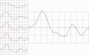
Figure 2. Sine synthesis. Functional sequence
on the left, last step on the right.
In the above figure, there is sine
synthesis sketched. It is possible to use it for imitating mountain range profile.
J. F. Blinn published 2D texturing technique based on Fourier synthesis in
1976. Anyone can play with explicit functions and get own results in one or two
dimensions.
We gathered that creating textures
from explicit functions in 2D is more complex than in 1D. See [boro00] for our
attempts to get natural-looking patterns.
Texture synthesis as a creative
process is sometimes understood like playing with explicit functions and
geometry to shape desired pattern. This approach is often called magic with
numbers. Steven Worley in [Ebert94] writes about toolbox functions. These
are set of functions used by a graphic artist, experienced in geometry, to form
the pattern. Textures like detailed honeycomb can be created this way.
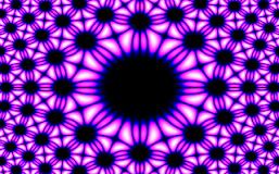
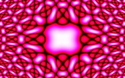
Figure 3. Formulas of type sin( f(x), g(y)
) were used to get these patterns.
We had played with goniometric
functions in raster. Two sample images are shown in the figure above. Both
pictures have 320x200 texels. Program generating these pictures made one pass
throughout whole texture space and defined a color from palette in each texel.
Even both patterns can be described as surfaces defined by explicit functions,
we visualized them with implicit algorithm: each point in raster was inquired
for the value. This way we could also visualized any implicit surface,
i.e. surface defined by the equation below.
Equation
(2). f(x) = 0
We now want to point out complexity
of texture generation. Under the term texture generation we mean a
process of running texture synthesis program on hardware. If program generating
textures on Figure
3 runs on one processor, it will need to perform
64000 computations on different input data. If we had parallel machine, program
can do 64000 computations at once (Simple Instruction Multiple Data; SIMD
principle). Anyway, it still requires the same computational time, because the
algorithm runs in one step, in which Equation (1) is computed
per texel. Solving this equation is atomic process, in general.
Parallel machines are more suitable
for problems of greater time complexity, where evolution of texel value is
necessary.
Fractals
Fractals are very popular example of
procedural modelling. Since there were many books published on this topic, we suppose
reader is acknowledged with fractal geometry. In [Ebert94], fractal shields are
discussed as the application suitable for terrain simulation. Hundred years
ago, diagrams like von Koch’s snowflake were studied. In the 1970’s, Benoit
Mandelbrot published his work. His name is linked with the famous set in 2D
plane.
Dragon curve or von Koch’s snowflake
are examples of hardly rasterized patterns. They consist of miscellaneously
angled links in planar area. Vector graphics (e.g. turtle graphics) is needed
for proper visualization.
Anyway, there are fractals with
raster nature. For instance, mid-point displacement algorithm also known as diamond algorithm can be easily modified
for grid of size 2nx2n.


Figure 4. Two sample outputs of modified diamond
algorithm
Original diamond algorithm is well
described in [diamond]. Purpose is to generate random 3D shield resembling
mountain. It relies on dynamically constructed grid.
Our slightly modified diamond
algorithm runs on static grid, which is a rectangular lattice. We implemented
the algorithm in 2D, using colour instead of height. We had to take care of the
grid size and stopping of the recursion. Hence, most suitable grid size is 2nx2n
for n steps. Results of our diamond algorithm are shown above.
Noises
It can be said, that much of
randomness in procedural modelling is due to involving some noise function into
the algorithm. First person revealing power of noises in raster was Ken Perlin.
He set a lattice of size n´m and assigned random values to each node. To get noise value in
arbitrary point in the plane, linear combination of values from 4 nodes nearest
to it are interpolated. This is called two-dimensional Perlin noise.
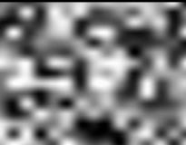
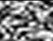
Figure 5. Perlin noise on 15x15 grid. Bicubic
interpolation on the left, compound bilinear on the right.
In the figure above reader can see
two exapmles of Perlin noises. They differ in the interpolation used. If we
displayed only 15x15 lattice defining the Perlin noise (shrunk so no blank
spaces left there), just 2D white noise would be seen.
Definition of 2D noise consists of
three requirements:
(1) Noise is statistically invariant according to translation
(2) Noise is statistically invariant according to rotation
(3) Noise is chaotic (sharp frequency spectrum in Fourier domain)
Perlin noise satisfies all of them.
We are using noise of different
nature than Perlin’s in our work. We call it averaged noise. Rather than
defining it numerically, we describe its algorithm.
In the first step, rectangular grid
is filled in with random values. In every next step, value for each texel is
recomputed. It is set to average of 3x3 values from the neighbourhood (texel
itself is also considered). Applying one step, nothing special would be seen.
Applying more steps, interesting pattern will start to form.
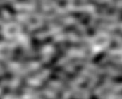
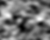
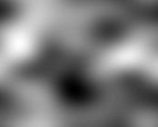
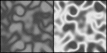
Figure 6. Averaged Noise. Three stages of
evolution were captured.
Figure above shows three stages (from
left to right) of the noise evolution. Greyscale palette is used to highlight
global minimum/maximum values on the grid. Bellow is the algorithm. It is
written in rough form, for the implementation see Appendix A.
Input: grid, one texel is referenced by
texel[x,y]
Step 0: for all meaningful x,y:
texel[x,y] := random value
Step i: for all meaningful x,y:
texel[x,y] := k * texel[x,y]
How to compute k in the step i:
k:= 0;
for i:= -1 to 1 do
for j:= -1 to 1 do
k := k + texel[x+i,y+j];
Understanding grid as a matrix, each
step of the algorithm is convolution. This is the convolution matrix:

It is an identity matrix multiplied
by the constant. Hence, averaged noise satisfies noise function requirements
(1) and (2). After stopping the algorithm in the step s, requirement (3)
also satisfied. To make a clear proof, choice of s would depend on the
grid size.
First step of the algorithm is 2D
white noise. Whole system converges into stable pattern of an overall average
value.
Matrix K can be altered. Then
we get anisotropic effects. Anyway, sum of its members must be equal to 1 under
all circumstances.
Let us compare 2D Perlin noise to
averaged noise. Perlin noise requires mesh to be defined. Interpolation must be
used for texels inside the mesh.
Averaged noise is any pattern from
algorithm described above. Time of evolution define the scale; more steps are
applied, greater the blurs are. It is due to isotropic diffussion. It can be
used for procedural terrain generation (see Appendix A). However, noise alone is not suitable for generating mountain
ranges, because averaged noise is defined implicitly. Matrix K changes
only local properties of the pattern, it can not affect isotropism in global
scale. On the other hand, mountain ranges are most simply defined as polylines.
Polylines are explicit objects, whereas noise is implicit object. What about
setting mountain range as polylines, and subsequently applying the averaged
noise?
Reaction-Diffusion
Although it is one of the youngest
techniques used in texture synthesis, Alan Turing formalized reaction-diffusion
(RD) already in 1952. It described chemical processes on cellular level in the
field of embrional morphogenesis. Chemicals acting in the process were named morphogens.
For detailed introduction into reaction-diffusion for computer graphics we
refer reader to [Witkin91] and [Turk91].
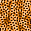
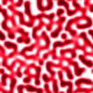
Figure 7. Two outputs of the same RD system.
Structural difference is due to different initial states.
RD can help to create mammalian coat
patterns and other amazing images. Many articles including this topic appeared
in 1990’s. We experimented with RD in [Boro00].
There were two main problems in RD
according to computer graphics:
(1) How to implement RD equation on computers
(2) What equations are useful for computer graphics
Let us shortly discuss the first
problem. In biology, RD is viewed as a space of cells interchanging their
content. Cell is an irregular object. It interacts only with its closest
neighbours.
Figure 8. Reaction and Diffusion.
There are 2 phases of RD step sketched
in Figure 8. First is reaction, second one is diffusion. Diffusion is the only
mechanism how can cell communicate with others.
In computer graphics, most effort was
taken on efficient cell communication. Simplest RD systems were rectangular
lattices where cells performed diffusion in parallel. Cell had 4 or 8
neighbours in this case. Other cell space topologies were also studied. Very
useful was an idea of attaching cell space to 3D model and simulation of RD
directly on that model. There are lot of papers considering texture synthesis
on arbitrary surfaces using any reasonable procedural technique, now.
2. Texture Synthesis Applications
We overviewed 4 famous classes of
procedural textures in the previous section. There is lot of software
applications for each technique as well as systems combining them. Standalone
authoring tools allowing to create user-defined procedural textures became
popular, recently. They usually output finalized texture in some standart picture format. Our work can be considered as a development
of such authoring tool.
However, we must
be interested in what are the other possibilities. Let us recall some ideas
relevant to texture synthesis.
Cellular Automaton Projects
There are many scientific groups
solving problems on cellular automaton. These are efficiently parallelized
virtual lattices suitable for the field of computer simulation, in which
procedural texture creation belongs to.
Shaders Inside Renderers
Before fast hardware shading, there
were several renderers capable of software shading. Shaders were incorporated
into the rendering pipeline, making users dependent on particular system.
However, shading process usually consisted of simple texture layering by the
mid-nineties. There was a possibility to import own textures. With increasing
importance of texture synthesis, shaders began to be independent ([Porter98],
Blue Moon Rendering Tools, etc.).
Plugin Systems
There are cutting-edge rendering and
modelling systems offering comfort of modularity (we mean plugin systems). One
can write its own shader and experiment with texture creation. Importance of
scripts (e.g. Python) and high-level languages (C/C++) arises. Implementing an
algorithm for different rendering systems at once is possible.
Authoring tools for texture synthesis
Totally independent authoring tool
for texture creators has one main advantage: graphic artist needs to know
nothing about scene geometry. Flat textures are constructed, instead. Output of
such system is exported to software/hardware renderer.
CG
One of the market leaders in PC
graphic cards machinery introduced shading language called “CG” in 2002. It is
based on the well-known C language. We think that this could be the way of
writing shaders in the future, because shader developer is not disturbed with
hardware properties.
Reader can dispute, that there are
other shading standards on the market. Yes, CG is not the only one. But it is a
very demonstrative example of how important for the rendering pipeline shading
process is.
What texture synthesis techniques are
suitable to implement in CG? The answer should be: any. But the real question
is: how much effort is needed for coding particular procedural texture? And the
answer depends on:
·
Knowledge of CG
·
Decision of shader type (vertex/pixel)
·
Visualization (color texture/bump
map/displacement/opacity/…)
·
Debugging tool
Current drawback of CG is that
although it is declared as hardware independent, one has to have a particular
hardware before running CG runtime. Otherwise, developing and debugging CG code
could be unproductive.
3. Short Introduction to Cellular Automata
We describe cellular automata (CA)
according to texture synthesis in this section. Reader would find more CA
applications related to computer graphics in [Takai].
Cellular automaton is system
consisting of:
·
Finite CA space
·
Initial state
·
Rules of evolution
Element of CA space is called cell.
Each cell is in one of its states. Evolutional rule tells cell how to behave.
Computation on cellular automaton starts at initial step, where initial states
are assigned to cells. Next steps are computed using evolutional rules. They
are same for each cell. Cellular automaton is SIMD (Simple Instruction Multiple
Data) parallel system, indeed.
Common CA definition citated from
[NIST]:
Definition: Usually a two-dimensional organization
of simple finite state machines whose
next state depends on their own
state and the states of their eight closest neighbors. In general the machines
may be arranged in meshes of higher or lower dimension, have larger
neighborhoods, or be arbitrarily complex processors.
Note: Conway's game of Life is
probably the most well known instance of a cellular automaton.
Cellular Automaton as Parallel System
We said that cellular automaton is
SIMD parallel system. Such systems are studied on parallel machines,
which solve problems by dividing them into smaller pieces. On the other hand,
we have distributed systems.
Distributed system is a net, where
each node computes its part of the problem. Difference between parallel systems
and distributed systems is that we have to know number of processors in the
parallel machine, whereas distributed system can be dynamic net. Demonstrative
example of distributed system is radio sample analysis for the SETI project
[SETI@home]. Anyone having an access to the Internet can join.
4. Binary CA
Simplest instance of cellular
automata are binary cellular automata. We wanted to know, what textures could
this category yield. 4-neighbourhood binary CA was chosen for our experiments.
Texture domain consists of rectangular lattice with torus topology
(illustration on Figure 1), here. Cell is either in the state
0 or in the state 1.
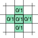
Figure 9. Cell and its 4-neighbourhood in the
binary CA
32 bits define program for the cell,
because next state of the cell depends on its own state plus state of 4
neighbours. Hence, our binary CA defines 232 (4 294 967 296)
programs. We wanted to know, how many of these programs define interesting
patterns/animations.
We developed an application, which
interprets arbitrary program (32 bits on input) on binary CA. White noise is
set as the initial state. After interpreting program in each state, CA space is
visualized: black color is associated to state 0, white color to state 1.
Program interpretation is so fast, that the system visualization is fluent
animation.
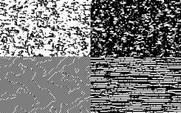
Figure 10. Textures created by randomly
generated programs on binary CA
Typing binary programs manually
wasn’t very comprehensive, therefore we decided to generate the programs
randomly. This method showed us surprising results: one can see amount of
interesting patterns/animations between dull pixel formations! Even simple
reaction-diffusion textures may be found there (see Figure 10 for sample outputs). We estimated, that about 1 from 5 randomly
generated programs gives some attractive pattern. Of course, what is and wat is
not attractive depends on the viewer’s attitude (more in [boro00]).
To sum up, animation on
4-neighbourhood binary CA can be specified by cell program and initial state.
We write source code for cell program as 32bit vector. In the initial state,
random binary is set to the cell. This method yields many binary animations. If
we run the same program on large grid (40x40) with different initial states, we
get statistically same animations. Choice of particular white noise does
not influence the pattern/animation characteristics, it influences only the
amount and positions of its typical local properties. Hence, all statistically
same animations can be treated as one binary evolutional texture. In the
other words, 32bit vector specifies any binary evolutional texture runable on
our binary CA.
Source code for the cell program may
be represented as 32bit number. Therefore, 4 294 967 296 binary evolutional textures
are defined on our binary CA. Moreover, source code of the program can be
created randomly.
5. Adding more complexity into binary CA
Averaged noise from Figure 6 cannot be defined on CA. More complexity is needed here. Thus we
extended the power of binary CA by considering 6 floating-point variables
instead of one binary. We get much more than binary textures, because 6
decimals specify more states than 1 bit. For example, all famous
reaction-diffusion systems use no more than 6 variables per cell.
But, there was a question: how should
the cell program look like? If we apply same method as in the previous section,
we get very strange source code. It would consist of 26 x 5 x
sizeof(decimal) x 8 bits , thus it would not be writable/readable.
Additionally, no interpreter of such source code would be fast enough.
We specified language, called TxrLan
in this document (abbreviation from Texture Language), as a solution more
comfortable for a texture creator. It is language made of conditionals. Program
is list of up to 6 rules – one rule for each variable. Rule defines next
variable’s value. Rather than specify the language precisely, we demonstrate
its nature on the example.
Averaged noise implemented in TxrLan
Suppose convolution noise with this
convolution matrix:
The matrix defines anisotropic
averaged noise. We need only one cell variable. TxrLan user has to decide, what
pattern will start the evolution. In our solution, up to timestep 3, random
value is assigned to the cell. Then, convolution is made by averaging the left,
upper and the cell own variables.
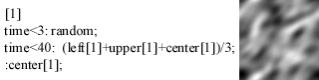
Figure 11. Example of TXR LAN: code on the left, visualization on the right.
Source code in the above figure may
be read line–by–line as follows:
This is rule for my 1st variable
if (time < 3) then variable := random,
else if (time < 40) variable := average of neighbours’ and my 1st
variables,
else variable := my 1st variable
Function random outputs random
floating-point value from interval á0,1ñ. Interpretation of exampled source code begins by a white noise.
Blending of neighbouring values during the algorithm causes kind of wax melting
effect. Difference to average noise as implemented in Appendix A is that this pattern is anisotropic. Resulting animation shows
average noise shifting in downright direction. We did not study, if pattern in Figure 11 is equivalent to isotropic average noise.
Discussion on TxrLan
No language is useful without
practical applications. What are the applications suitable for TxrLan? Reader
should know these:
·
Binary evolutional textures
·
Reaction-diffusion
·
Convolution noises
We know them as texture synthesis
techniques. They can be viewed as numerical problems, too. TxrLan can help to
solve lot of other problems ([boro00]).
There is another question: what is
TxrLan not suitable for? We tried to implement diamond fractal algorithm, but
the source code was too long, thus unreadable. We gathered that any phenomenon
described explicitly is not suitable for TxrLan. Rather than theory, we
introduce an example.
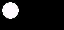
|
Circle, radius 15
[1]
sqrt(sqr(x-20)+sqr(y-20)) < 15.5: 1;
:0;
|

|
Figure 12.
Circle coded in TxrLan
Above is source code for one circle.
Although all cells are running the same program, majority has the same state
during the evolution. Why? There are two reasons: spatial and temporal.
Spatial
Let us freeze the time. Circle is an
explicit object. Only inner cells specify it. Outer cells are not interesting.
Another object can be defined outside the circle.
Temporal
Let us forget the space and consider
one cell only. When this cell changes its state? Possibly in the first step,
never after then.
We have no explanatory capabilities
to precisely abstract the idea. We can just say, that circle (example of object
explicitly defined in space and time) wastes power of TxrLan interpreter.
Let us introduce small analysis on
what does it mean to implement program optimally on CA. We remark, that TxrLan
is an instance of CA.
Suppose problem p formally
defined on CA. Develop a program, which solves p on cellular automaton.
Start the program. Call the situation in which cell is chaning its state one
swap. Measure, how many swaps are during the program execution. Denote the
result as M(p).
Observation:
Great value of M(p) indicates,
that problem p is effectively solved on CA.
In our circle example, M(circle)
= 177 (approximated as p ´ 7.52).
In the example from Figure 11, M(avenoise) = maxX x maxY x 40 (maxX, maxY
specify grid size). Notice, that M(avenoise) is maximal possible. It
proves, that program from Figure 11 solves averaged noise
problem optimally.
Abstraction:
Problem p is optimally
implemented on CA, if and only if M(p) = maximal possible.
This was our analysis. It looks fine,
but we used language of computer graphics rather than parallel systems. Theory of
parallel computing was based in [Jaja92]. It assumes that reader is educated in
sequential programming. Our analysis was not influenced by sequential
programming.
Conclusion
We believe that reader understood our
idea of joining CA and texture synthesis. If there is a demand, we will try to
develop language more suitable for graphic artists than TxrLan. This language
would be structural, i.e. it would allow to use variables as required. Source
code would be far more readable.
We excuse for accuracy in this
document. We wanted to describe the matter rather than formalize partial
problems.
We would strongly appreciate hearing
any comments from interested reader. Author’s current e-mail address is:
peter.borovsky@fractal.dam.fmph.uniba.sk
6. Appendices
This document is describing our work
in the written form. Reading it is sufficient for people curious about
procedural textures, CA or related topics. All examples in the document are
static images. For closer understanding of dynamic phenomena, software
applications and/or animations should be seen. Therefore we collected our
experimental software applications and made it available onto accompanied CD.
All applications should run under
Windows98/200/NT operating systems. Some of them where originally developed
under MS-DOS.
For closer understanding, runable
programs must be seen.
There are our source codes and
executables available on the CD. There are also www pages and other materials
related to the theme, which are properties of their authors.
Appendix A
We described averaged noise in this
paper. However, any algorithm description is not a definition. Therefore we
print out following C++ source code. It is located at
sources \ averaged noise \ main.cpp
on the accompanied CD. Knowledge of
C++ is necessary to understand the code. It was written with attention to
readability.
Compiled application runs 8.5 seconds
on Athlon XP 1600 CPU. It executes 50 convolution steps on 64000 texels. Hence,
one texel value is recomputed in 0.00000265625 seconds. Most time consuming
operation is texel visualization.
//---------------------------------------------------------------------------
/*
averaged noise definition
*/
/*
first_step() makes 2D white noise.
step() performs one convolution step on pfSpace[][].
TfrmMain::show_space() visualizes one step.
Algorithm is triggered by TfrmMain::Trigger()
function.
*/
#include <vcl.h>
#pragma hdrstop
#include "main.h"
//---------------------------------------------------------------------------
#pragma package(smart_init)
#pragma resource "*.dfm"
TfrmMain *frmMain;
#define MAX_X 320
#define MAX_Y 200
float pfSpace[MAX_X][MAX_Y];
float pfBackup[MAX_X][MAX_Y];
//---------------------------------------------------------------------------
first_step()
{
randomize;
for
(int i = 0; i < MAX_X; i++)
{
for (int j = 0; j < MAX_Y; j++)
{
pfSpace[i][j] = rand() % 1000;
}
}
}
step()
{
//
backup space
memcpy( pfBackup, pfSpace, MAX_X * MAX_Y * sizeof(float) );
//
make lattice convolution
for
(int x = 0; x < MAX_X; x++)
{
for (int y = 0; y < MAX_Y; y++)
{
// compute convolution for texel [x,y]
float f = 0;
for (int i = -1; i <= 1; i++)
{
for (int j = -1; j <= 1; j++)
{
f += pfBackup[(x+MAX_X+i) % MAX_X ][(y+MAX_Y+j) %
MAX_Y ];
// rollover causes seamless effect
}
}
f /= 9; // 3x3 neighbourhood is considered
pfSpace[x][y] = f;
}
}
}
TfrmMain::show_space()
{
//
get minimum/maximum from the space
float fMin = 100000;
float fMax = -1;
for
(int x = 0; x < MAX_X; x++)
{
for (int y = 0; y < MAX_Y; y++)
{
if ( pfSpace[x][y] < fMin )
{
fMin = pfSpace[x][y];
}
else if ( pfSpace[x][y] > fMax )
{
fMax = pfSpace[x][y];
}
}
}
//
get global disperse
float fDisp = fMax - fMin;
//
show space
for
(int x = 0; x < MAX_X; x++)
{
for (int y = 0; y < MAX_Y; y++)
{
float f = (pfSpace[x][y] - fMin) / fDisp;
Canvas->Pixels[x][y] = RGB( 255.0 * f, 255.0 * f, 255.0 * f);
}
}
}
//---------------------------------------------------------------------------
void __fastcall TfrmMain::Trigger(TObject
*Sender)
{
// 1st
step is setting of random values
first_step();
//
do 50 steps of evolution
for
(int i = 0; i < 50; i++)
{
step();
show_space();
lbStep->Caption = i+1;
Update();
}
}
//---------------------------------------------------------------------------
We used average noise in programs for
generating earth relief procedurally. One of our executable can be found on the
CD in
executables \ averaged noise\ relief
It is an old-fashioned computer game
written in Borland Pascal environment under MS-DOS operating system. We
encourage reader to run it, because there is a step–by–step procedural terrain
generation animated well.
Appendix B
TxrLan is interpreter of language we
proposed in [Boro00]. Input is any
text file with a cell program. Cell program consists of rules – one rule for
one variable. Interpreter can be found on the CD in
First TxrLan
interpreter was developed in 1999, stable version 1.6 was presented in 2000.
Recently we upgraded the software for presentation purposes. It is located in
executables \ TxrLan
There are many
example source codes. We encourage reader to play with them. Changing
appropriate constant sometimes leads to unexpected and still interesting
animation. Here follows samples. Source codes are on the left, outputs captured
as static images are on the right. In the third sample only 2 from 3 morphogens
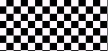
are shown.
|
chessboard, 8x8 px fields
[1]
mod(y,16) < 8:
mod(x,16) < 8: 1;
:0;
mod(x,16) >7: 1;
:0;
|
|
|
Circle, radius 15
[1]
sqrt(sqr(x-20)+sqr(y-20)) < 15.5: 1;
:0;
|
|
|
Reaction-diffusion system, 3 morphogens
[1]
time<2: 4;
:center[1]+0.03125*(16-center[1]*center[2])+0.25*(left[1]+right[1]+upper[1]+lower[1]-4*center[1]);
[2]
time<2: 4;
:center[2]+0.03125*(center[2]*(center[1]-1)-center[3])+0.0625*(left[2]+right[2]+upper[2]+lower[2]-4*center[2]);
[3]
time<2: 12+random*0.05-0.025;
:center[3];
|
|
Appendix C
At [CG], we found a contribution of RD
coded in CG. Interested reader would found the code on accompanied CD as
www \ RD in CG.htm
We do not print it out. The purpose
of this appendix is to show a difference between shading language such as CG
and language for texture synthesis. In a shading language program, much of an
effort is taken on visualization. Our TxrLan does not care about visualization.
Therefore, reaction-diffusion system can be coded in couple of lines as showed
in Appendix B.
TxrLan has main disadvantage against
CG in debugging. We tried to debug programs under construction by assigning
special values to examined cells. It worked, but for huge source codes some
user-friendly debugging is more convenient.
References
[Ebert94] D.
S. Ebert, F. K. Musgrave, D. Peachey, K. Perlin, S. Worley: Texturing and Modeling: A Procedural
Approach, Academic Press, Cambridge, 1994.
[Witkin91] A.
Witkin, M. Kass: Reaction-Diffusion Textures, in W. Sedeberg, editor: Computer Graphics (SIGGRAPH ’91 Proceedings),
volume 25, pp. 299-308, 1991.
[Turk91] G.
Turk: Generating Textures on Arbitrary Surfaces Using Reaction-Diffusion, in W.
Sedeberg, editor: Computer Graphics
(SIGGRAPH ’91 Proceedings), volume 25, pp. 289-298, 1991.
[Jaja92] J.
Jájá, An introduction to Parallel Algorithms, Addison-Wesley (ISBN
0-201-54856-9), 1992
[Talia00] D.
Talia: Cellular Processing Tools for High-Performance Simulation, in: IEEE Computer, volume 44, September
2000.
[Boro00] P.
Borovský, Procedurálne Textúry,
Diploma thesis, MFF UK, 2000
[DarkTree] Darkling
Simulations: http://www.darksim.com
[Takai] Graphics
Applications of Cellular Automata: http://madeira.cc.hokudai.ac.jp/RD/takai/automa.html
[NIST] Dictionary
of Algorithms and Data Structures: http://www.nist.gov/dads/HTML/cellulartmtn.html
[SETI@home] SETI@home
experiment: http://setiathome.ssl.berkeley.edu/
[diamond] Mid
Point Displacement Algorithm: http://www.lighthouse3d.com/opengl/terrain/index.php3?mpd2
[CG]
CG shaders: http://www.cgshaders.org/
[Boro00C] Evolutionary Textures: http://www.cg.tuwien.ac.at/studentwork/CESCG/CESCG-2000/PBorovsky/index.html
Hyperlinks validity checked at 2003-feb-13. Some of web
pages can be found offline on accompanied CD.